Learning Excel

Welcome to Learning Excel!

If you have questions or comments, please click the comment click below. Comments are moderated.

Remember, you are attempting to learn Excel without an instructor. This can be a frustrating process! Do not give up!

Also, there are many ways to accomplish tasks in Microsoft applications. In most exercises, you will only learn one way to complete the task.

You will find the notes for this class at http://excel.schtuff.com.

The Excel instructional videos are hosted on vimeo.com.

Slideshow.

Begin by viewing the slideshow, IntroductiontoExcel_webversion.ppt, at http://excel.schtuff.com/introductiontoexcel_webversion_ppt.

ClipArt.

1. Click on Insert menu.
2. Click on Picture.
3. Click on ClipArt.
4. The Insert Clip Art task pane will open on the right-hand of the screen.
5. Click in the Search text box.
6. Type in a word, such as pen, frog, etc.
7. Click Search.
8. The task pane will show the results of your search.
9. Choose an image and click on the image.
10. To move the image, click and drag the image.

Notes are located at at http://excel.schtuff.com/excel_clipart_doc
.

Cell Border.

1. Highlight cells with data.
2. Open the Format menu.
3. Click on Cells.
4. Make sure you are viewing the Border window. If not, click on the Border tab.
5. Under Presets, choose the Outline option.
6. Look at the Preview box.
7. Under Presets, choose the Inside option.
8. Look at the Preview box.
9. Remove the Top Border.
10. Look at the Preview box.
11. Remove the Left Border.
12. Click OK button.

Borders on Vimeo

Notes are located at at http://excel.schtuff.com/excel_cell_border_doc
.

Merge and Center.

1. In a new spreadsheet, in Cell A1 type This is the title.
2. In A2, type first.
3. In B2, type second.
4. In C2, type third.
5. In D2, type fourth.
6. In E2, type fifth.
7. In F2, type sixth.
8. Click cell A1 so that it is active. Center the contents of the cell by click the Center button on the toolbar. Notice that This is the title is centered in its cell, but not centered over columns A through F.
9. Highlight cells A1 through F1.
10. Click the Merge button on the toolbar.

Merge and Center on Vimeo

Notes are located at at http://excel.schtuff.com/excel_merge_and_center_doc
.

Graphs and Charts.

1. Enter the following data. (See image below)

Top Cheese Spread/Ball Brands, 2003

($ mil.) Share
Alouette 5.19 9.27
Kaukauna 4.65 8.31
Price 3.6 6.43
Wispride 2.78 4.97
Private label 7.35 13
Other 32.4 58.02
100

MarketShare Report 2005

2. Select Insert Menu. Choose Chart.
3. Make sure the Standard Types tab is selected. If not, click the Standard Types tab.
4. Under Chart Types select Pie.

5. Click Next.
6. Make sure the insertion point is blinking in the Data range text box.

7. On the worksheet, highlight cells A4 through A9.
8. Hold the CTRL key down and also highlight cells C4 through C9. Let go of the CTRL key.

9. Click Next.
10. Make sure the Title tab is selected. If not, click the Title tab.
11. In the Chart Title textbox, type Top Cheese Spread/Ball Brands 2003.

12. Click Next.
13. Make sure that As object in: Sheet1 is selected.

14. Click Finish

Notes are located at at http://excel.schtuff.com/excel_charts_doc

and

http://excel.schtuff.com/excel_graph_doc

Absolute Cells.

1. In cell A1, type 5.
2. In cell A2, type 10.
3. In cell A3, type =A1+A2 (Press Enter)
4. Click cell A3 so that it is active.
5. Select the Edit Menu. Choose Copy.
6. Highlight cells A4 through A14.
7. Select the Edit Menu. Choose Paste.
8. In cell B1, type 5.
9. In cell B2, type 10.
10. In cell B3, type =$B$1+B2 (Press Enter)
11. Click cell B3 so that it is active.
12. Select the Edit Menu. Choose Copy.
13. Highlight cells B4 through B14.
14. Select the Edit Menu. Choose Paste.

Notes are located at at http://excel.schtuff.com/excel_absolute_doc
.

Sorting.

1. Type the following information
Brad Brad's phone
Andy Andy's phone
Mark Mark's phone
Scott Scott's phone
Steve Steve's phone
Sam Sam's phone
Justin Justin's phone
Brian Brian's phone

2. Notice that Column A has the person’s name and Column B has the person’s phone (ie. Brad’s phone). Each row is considered a record.
a. If we only sort Column A. The names will not match the phone numbers. We need to sort the contents of Column A with the contents of Column B.
3. Highlight Column A and Column B. This can be done by clicking and dragging on the column headers.
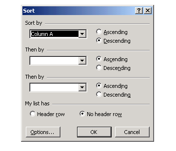
4. Select the Data Menu. Choose Sort.

5. We want to sort the records by the first name so the default, Column A, is correct. We will also sort A-Z so the default Ascending is correct.

6. Click OK.

7. The records should now be sorted alphabetically A-Z by their first names.
Andy Andy's phone
Brad Brad's phone
Brian Brian's phone
Justin Justin's phone
Mark Mark's phone
Sam Sam's phone
Scott Scott's phone
Steve Steve's phone

8. Make sure your data is highlighted. Select the Data Menu. Choose Sort.

9. Change the default to Descending. This will sort the first names Z-A.

10. The records should now be sorted alphabetically Z-A by their first names.
Steve Steve's phone
Scott Scott's phone
Sam Sam's phone
Mark Mark's phone
Justin Justin's phone
Brian Brian's phone
Brad Brad's phone
Andy Andy's phone

11. Click on the Row 1 heading.
12. Select the Insert Menu. Choose Row.
13. In cell A1, type Name. (This is a heading)
14. In cell B1, type Phone. (This is a heading)
15. Highlight Column A and Column B.
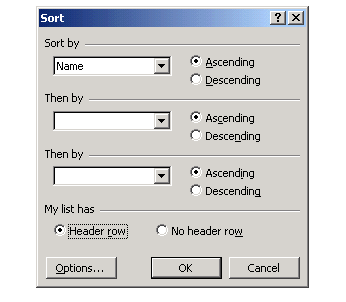
16. Select the Data Menu. Choose Sort.
17. In the Sort Window, select Ascending.
18. Under My list has, select Header Row.
19. Click OK.

20. Your headers, Name and Phone, should still be in cells A1 and B1.

Sorting on Vimeo

Notes are located at at http://excel.schtuff.com/excel_sorting_doc
.

Insert Function.

1. Enter the following numbers in cells B1 through B7
234
123
234
534
523
1234
3245

2. In cell A8 type Sum

3. In cell A9 type Average

4. In cell A10 type Maximum

5. In cell A11 type Minimum

6. In cell A12 type Count

7. Click the cell B8. Make sure that this cell is active.
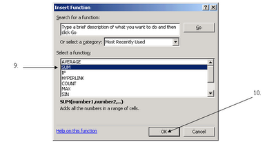
8. Click the Insert Function button.

9. In the Insert Function window, choose SUM.

10. Click OK.

11. The default range, B1:B7, is correct. Do not change anything.

12. Click OK.

13. The number in the cell should be 6127. This is the sum of the numbers in cells B1 through B7. The formula bar should read =sum(B1:B7) .

14. Click the cell B9. Make sure that this cell is active.
15. Click the Insert Function button.

16. In the Insert Function window, choose AVERAGE.

17. This time the default range is not correct. Instead of B1:B8 (cells B1 through B8), we want cells B1:B7 (the original numbers typed in).
Change the cells by changing the default to B1:B7 with the keyboard or highlight the correct range on the worksheet.

18. Click OK.

19. The number in the cell should be 875.2857. This is the average of the numbers in cells B1 through B7. The formula bar should read =average(B1:B7) .

Insert Function on Vimeo

Notes are located at at http://excel.schtuff.com/excel_insert_function_button_doc
.